http://quantstart.com/articles/Basics-of-Statistical-Mean-Reversion-Testing
dxt=θ(μ−xt)dt+σdWt
Δyt=α+βt+γyt−1+δ1Δyt−1+⋯+δp−1Δyt−p+1+ϵt
DFτ=γ^SE(γ^)

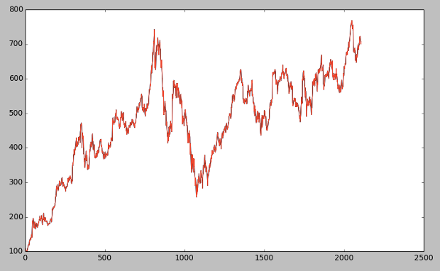
Google price series from 2000-01-01 to 2013-01-01
Var(τ)=⟨|log(t+τ)−log(t)|2⟩
⟨|log(t+τ)−log(t)|2⟩∼τ
⟨|log(t+τ)−log(t)|2⟩∼τ2H
BASICS OF STATISTICAL MEAN REVERSION TESTING
So far on QuantStart we have discussed algorithmic trading strategy identification, successful backtesting,securities master databases and how to construct a software research environment. It is now time to turn our attention towards forming actual trading strategies and how to implement them.
One of the key trading concepts in the quantitative toolbox is that of mean reversion. This process refers to a time series that displays a tendency to revert to its historical mean value. Mathematically, such a (continuous) time series is referred to as an Ornstein-Uhlenbeck process. This is in contrast to a random walk (Brownian motion), which has no "memory" of where it has been at each particular instance of time. The mean-reverting property of a time series can be exploited in order to produce profitable trading strategies.
In this article we are going to outline the statistical tests necessary to identify mean reversion. In particular, we will study the concept of stationarity and how to test for it.
Testing for Mean Reversion
A continuous mean-reverting time series can be represented by an Ornstein-Uhlenbeck stochastic differential equation:
Where θ is the rate of reversion to the mean, μ is the mean value of the process, σ is the variance of the process and Wt is a Wiener Process or Brownian Motion.
In a discrete setting the equation states that the change of the price series in the next time period is proportional to the difference between the mean price and the current price, with the addition of Gaussian noise.
This property motivates the Augmented Dickey-Fuller Test, which we will describe below.
Augmented Dickey-Fuller (ADF) Test
Mathematically, the ADF is based on the idea of testing for the presence of a unit root in anautoregressive time series sample. It makes use of the fact that if a price series possesses mean reversion, then the next price level will be proportional to the current price level. A linear lag model of order p is used for the time series:
Where α is a constant, β represents the coefficient of a temporal trend and Δyt=y(t)−y(t−1) . The role of the ADF hypothesis test is to consider the null hypothesis that γ=0 , which would indicate (with α=β=0 ) that the process is a random walk and thus non mean reverting.
If the hypothesis that γ=0 can be rejected then the following movement of the price series is proportional to the current price and thus it is unlikely to be a random walk.
So how is the ADF test carried out? The first task is to calculate the test statistic (DFτ ), which is given by the sample proportionality constant γ^ divided by the standard error of the sample proportionality constant:
Dickey and Fuller have previously calculated the distribution of this test statistic, which allows us to determine the rejection of the hypothesis for any chosen percentage critical value. The test statistic is a negative number and thus in order to be significant beyond the critical values, the number must be more negative than these values, i.e. less than the critical values.
A key practical issue for traders is that any constant long-term drift in a price is of a much smaller magnitude than any short-term fluctuations and so the drift is often assumed to be zero (β=0 ) for the model.
Since we are considering a lag model of order p , we need to actually set p to a particular value. It is usually sufficient, for trading research, to set p=1 to allow us to reject the null hypothesis.
To calculate the Augmented Dickey-Fuller test we can make use of the pandas and statsmodels libraries. The former provides us with a straightforward method of obtaining Open-High-Low-Close-Volume (OHLCV) data from Yahoo Finance, while the latter wraps the ADF test in a easy to call function.
We will carry out the ADF test on a sample price series of Google stock, from 1st January 2000 to 1st January 2013.

Google price series from 2000-01-01 to 2013-01-01
Here is the Python code to carry out the test:
# Import the Time Series library
import statsmodels.tsa.stattools as ts

# Import Datetime and the Pandas DataReader
from datetime import datetime
from pandas.io.data import DataReader

# Download the Google OHLCV data from 1/1/2000 to 1/1/2013
goog = DataReader("GOOG", "yahoo", datetime(2000,1,1), datetime(2013,1,1))

# Output the results of the Augmented Dickey-Fuller test for Google
# with a lag order value of 1
ts.adfuller(goog['Adj Close'], 1)
Here is the output of the Augmented Dickey-Fuller test for Google over the period. The first value is the calculated test-statistic, while the second value is the p-value. The fourth is the number of data points in the sample. The fifth value, the dictionary, contains the critical values of the test-statistic at the 1, 5 and 10 percent values respectively.
(-2.1900105430326064,
 0.20989101040060731,
 0,
 2106,
 {'1%': -3.4334588739173006,
  '10%': -2.5675011176676956,
  '5%': -2.8629133710702983},
 15436.871010333041)
Since the calculated value of the test statistic is larger than any of the critical values at the 1, 5 or 10 percent levels, we cannot reject the null hypothesis of γ=0 and thus we are unlikely to have found a mean reverting time series.
An alternative means of identifying a mean reverting time series is provided by the concept of stationarity, which we will now discuss.
Testing for Stationarity
A time series (or stochastic process) is defined to be strongly stationary if its joint probability distribution is invariant under translations in time or space. In particular, and of key importance for traders, the mean and variance of the process do not change over time or space and they each do not follow a trend.
A critical feature of stationary price series is that the prices within the series diffuse from their initial value at a rate slower than that of a Geometric Brownian Motion. By measuring the rate of this diffusive behaviour we can identify the nature of the time series.
We will now outline a calculation, namely the Hurst Exponent, which helps us to characterise the stationarity of a time series.
Hurst Exponent
The goal of the Hurst Exponent is to provide us with a scalar value that will help us to identify (within the limits of statistical estimation) whether a series is mean reverting, random walking or trending.
The idea behind the Hurst Exponent calculation is that we can use the variance of a log price series to assess the rate of diffusive behaviour. For an arbitrary time lag τ , the variance is given by:
Since we are comparing the rate of diffusion to that of a Geometric Brownian Motion, we can use the fact that at large τ we have that the variance is proportional to τ in the case of a GBM:
The key insight is that if any autocorrelations exist (i.e. any sequential price movements possess non-zero correlation) then the above relationship is not valid. Instead, it can be modified to include an exponent value "2H ", which gives us the Hurst Exponent value H :
A time series can then be characterised in the following manner:
H<0.5 - The time series is mean revertingH=0.5 - The time series is a Geometric Brownian MotionH>0.5 - The time series is trending
In addition to characterisation of the time series the Hurst Exponent also describes the extent to which a series behaves in the manner categorised. For instance, a value of H near 0 is a highly mean reverting series, while for H near 1 the series is strongly trending.
To calculate the Hurst Exponent for the Google price series, as utilised above in the explanation of the ADF, we can use the following Python code:
from numpy import cumsum, log, polyfit, sqrt, std, subtract
from numpy.random import randn

def hurst(ts):
 """Returns the Hurst Exponent of the time series vector ts"""
 # Create the range of lag values
 lags = range(2, 100)

 # Calculate the array of the variances of the lagged differences
 tau = [sqrt(std(subtract(ts[lag:], ts[:-lag]))) for lag in lags]

 # Use a linear fit to estimate the Hurst Exponent
 poly = polyfit(log(lags), log(tau), 1)

 # Return the Hurst exponent from the polyfit output
 return poly[0]*2.0

# Create a Gometric Brownian Motion, Mean-Reverting and Trending Series
gbm = log(cumsum(randn(100000))+1000)
mr = log(randn(100000)+1000)
tr = log(cumsum(randn(100000)+1)+1000)

# Output the Hurst Exponent for each of the above series
# and the price of Google (the Adjusted Close price) for
# the ADF test given above in the article
print "Hurst(GBM):   %s" % hurst(gbm)
print "Hurst(MR):    %s" % hurst(mr)
print "Hurst(TR):    %s" % hurst(tr)

# Assuming you have run the above code to obtain 'goog'!
print "Hurst(GOOG):  %s" % hurst(goog['Adj Close'])
The output from the Hurst Exponent Python code is given below:
Hurst(GBM):   0.500606209426
Hurst(MR):    0.000313348900533
Hurst(TR):    0.947502376783
Hurst(GOOG):  0.507880122614
From this output we can see that the Geometric Brownian Motion posssesses a Hurst Exponent, H , that is almost exactly 0.5. The mean reverting series has H almost equal to zero, while the trending series has H close to 1.
Interestingly, Google has H also nearly equal to 0.5 indicating that it is extremely close to a geometric random walk (at least for the sample period we're making use of!).
While we now have a means of characterising the nature of a price time series, we have yet to discuss howstatistically significant this value of H is. We need to be able to determine if we can reject the null hypothesis that H=0.5 to ascertain mean reverting or trending behaviour.
In subsequent articles we will describe how to calculate whether H is statistically significant. In addition, we will consider the concept of cointegration, which will allow us to create our own mean reverting time series from multiple differing price series. Finally, we will tie these statistical techniques together in order to form a basic mean reverting trading strategy.
Related Articles
- Beginner's Guide to Quantitative Trading
- Best Programming Language for Algorithmic Trading Systems?
- Can Algorithmic Traders Still Succeed at the Retail Level?
- How to Identify Algorithmic Trading Strategies
- Installing a Desktop Algorithmic Trading Research Environment using Ubuntu Linux and Python
- Interactive Brokers Demo Account Signup Tutorial
- Securities Master Database with MySQL and Python
- Securities Master Databases for Algorithmic Trading
- Sharpe Ratio for Algorithmic Trading Performance Measurement
- Successful Backtesting of Algorithmic Trading Strategies - Part I
- Successful Backtesting of Algorithmic Trading Strategies - Part II
- Top 5 Essential Beginner Books for Algorithmic Trading